
Discussion
Discussion
While the central aspect of this work was computational, it also had an enzymological and biocatalytic background. In the meetings with many project partners, it became clear that initial rate analysis is most common and seldom questioned. But initial rate analysis has some underlying problems that make reproducing results and reanalysis of the data difficult. For example, there are no conventions on which reaction period has to be taken to calculate the initial rates. The two methods encountered during this work were, first, by taking the beginning, from the start of the reaction until some arbitrary time-point, ranging from only a few seconds up to 20 minutes. And second, to record the time-course data that might start with a lag phase and choose a linear part of arbitrary length with a sense of proportion. These choices are often not reported but can strongly influence the modelling results that might follow. Aside from not stating the interval from which the initial rates are calculated, information on the method to calculate the initial rates is often missing. Most partners work with Excel. If they have time-course data, they often use linear regression. But sometimes, their experimental setup only yields two or even just one data point, and the initial rates are calculated from these. Furthermore, initial rates always come with information loss. As a result, it is impossible to conclude the time-course from initial rates, and a lag phase at the beginning or incomplete substrate conversion visible at the end won’t find any attention. Jupyter Notebooks accompanying papers can mitigate these problems by documenting the whole calculation process. It’s recommended to start with visualisation to give readers an impression of the data before any calculations. The EnzymeML format encourages users to report all their raw data, making reanalysis possible. Since the EnzymeML format is still actively developed, this started a discussion on adding initial rates to the stored data. For completeness, this would also need the additional information aforementioned, at least of the time interval of the measurement.
In all scenarios, the modelling and curve-fitting were done with the well-established Python packages SciPy and lmfit. Simultaneously, the integration of other modelling tools into the EnzymeML toolbox, especially for COPASI [HSG+06] by Frank Bergmann and PySCeS [ORH04] by Johann Rohwer, advanced, which will further ease the modelling process of EnzymeML data. Where it was possible to compare results from lmfit with those of project partners, they were similar and within the same order of magnitude. Lmfit’s power compared to the software used by project partners is the simple expandability of the models. For example, the Michaelis-Menten kinetic could be extended with additional microkinetics resulting in coupled ODEs, as in scenarios 3 and 4. In contrast, other software provides a selection of models to choose from but is not extendable. The downsides of using lmfit are the need to provide initial values for the parameters; this can be hard, especially in the beginning, for less experienced users. Moreover, the results of lmfit for different initial values can be subject to strong fluctuations, and lmfit might only find local minima. On the other hand, the need to engage with the initial value selection and the selection of the model can make users more receptive to these problems, where they might not see these when presented with the results by software; this helps critical appraisal of the results and may lead to follow-up analyses.
Hiccups with Jupyter Notebooks.
Jupyter Notebooks, with their infrastructure, are beginner-friendly, but with extensive use, some stumbling blocks will be encountered. Jupyter Notebooks offer many options for formatting. Besides the standard markdown syntax, their markdown cells can incorporate additional HTML with javascript and latex syntax. However, these might be rendered differently or not at all in different environments such as Google Colaboratory, Binder or Jupyter-Lab. If possible, it is recommended to choose one and optimise the markdown for that. Another hurdle can be the format of Jupyter Notebooks in which they are stored and transferred. The raw representation of a Jupyter Notebook is a JSON schema containing much metadata, aside from code and markdown; this can lead to problems with version control. As of now, git has no good way to handle the differences in the JSON schema, which makes comparing versions for the user very hard and can, in some instances, lead to merge conflicts. However, the Jupyter project is already working on it and offers a git diff button in their classic and Jupyter-Lab environment, which only shows changes in the cells, not the metadata, as this is of interest for the user.
What makes the combination of EnzymeML and Jupyter Notebooks a FAIR way to model and report data?
First, EnzymeML documents and Jupyter Notebooks can be published on Zenodo [EuropeanOFNResearchOpenAIRE13] or in a DataVerse [Cro11] to get a DOI or uploaded to GitHub. There they are findable and accessible. Adding additional files to an EnzymeML document, such as a Jupyter Notebook, is also possible. For instance, DataVerses can be searched for specific metadata of EnzymeML documents. This way, one can easily find all relevant documents for a particular enzyme or reaction.
Jupyter Notebooks can be used interoperable with other tools. For example, it is possible to start an analysis in a Jupyter Notebook and then move on to another software and maybe come back to the Jupyter Notebook at a later point. The steps outside the Jupyter Notebook can be described in markdown cells. This Jupyter Notebook can still convey the whole analysis process. Jupyter Notebooks can also be part of a more extensive workflow, described in a workflow language, but this was not part of this work. Since a Jupyter Notebook is a coding environment, many different modelling tools can be run inside, such as COPASI and PySCeS. All scenarios were programmed in Python and used the PyEnzyme package to read, write and edit EnzymeML data; this facilitates the combination of Jupyter Notebooks and EnzymeML since no additional interface is needed.
As part of a well-developed infrastructure (Fig. 2), Jupyter Notebooks are easily reusable. Aside from writing and running a Jupyter Notebook on a local computer, they can be shared and run online. For example, in this report’s website version, all Jupyter Notebooks can be opened in Binder with just two clicks. It becomes more and more common practice for developers in research to share Jupyter Notebooks over Google Colaboratory. Some project partners also did this. With Binder and Google Colaboratory, Jupyter Notebooks can be run independently of your operating system. One of the biggest strengths is that no proprietary software is needed. Many project partners used proprietary software such as OriginPro and SigmaPlot for modelling. Apart from the obvious problem that others who do not have this software first have to find another software to reproduce the results, another software is often needed for further steps of the modelling process. Those software programs usually don’t have a consistent file format and can’t read or write EnzymeML or Excel files. Therefore interim results, such as initial rates, have to be copy-pasted, which is error-prone.
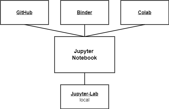
Fig. 2: Jupyter Notebook infrastructure, depicting diverse environments for programming and execution local and online.
The combination of EnzymeML and Jupyter Notebooks offers a great way to collaborate. For instance, at present, the collected data often spans multiple Excel files, some containing only raw data from the measuring instruments, others with unit conversions or whole calculations. As a result, it is hard to keep track of all relevant files, and for project partners, it can be hard to comprehend what has been done in the individual files, leading to further enquiries. EnzymeML offers a way to store all data in one file. Furthermore, the structure of Jupyter Notebooks with a combination of markdown and code cells makes all further steps, such as converting units and calculations, comprehensible for collaborators.